Markus Schläfli
Deep Learning from Scratch
Code for the post can be found here.
What surprised me most when implementing a neural network from scratch was how simple the fundamental idea behind deep learning - that is, the trivial form of a fully connected, feed-forward vanilla neural net - really is. And seeing as we’re talking about what’s been called the most important technical revolution in the last quarter century, I’d say that feels exciting!
I will skip the general motivation and basic overview for machine learning because: A) it’s damn hard to do (try it); B) others way more capable have done it - see 3Blue1Brown’s video; and C) if any particular section trips you up, you can get a personalized answer from any LLM for that specific part.
Let’s get to it.
Our problem - digit classification!
We’ll start where everyone starts in machine learning: recognizing hand-written digits. Given the large variation of what a handwritten digit could look like, it’s hard to imagine any form of if-else logic that you use to come up with a good recognition system.
For that, we’ll be using the MNIST dataset, consisting of 70’000 grayscale 28x28 pixel images of handwritten digits (0-9). It’s widely used because it’s simple enough to train on quickly, but also complex enough that you’ll want to start looking into using more advanced techniques. It’s the ‘hello world’ of machine learning and yet it requires the latest techniques to get >99% accuracy.
I’ll be skipping the code for loading the data in the post, but will provide it in the published code.
Model architecture
The neural network we are going to use is composed of multiple layers of fully connected neurons, meaning every neuron in a layer is connected to every neuron in the next layer. This is a Multilayer Perceptron (MLP) and happens to be one of the fundamental types in machine learning.
The image below shows what that looks like, but it only shows the connections from the first neuron for clarity (to extrapolate, just add imaginary lines from all the neurons below the first). The input layer consists of 8 neurons, which then feed into 2 hidden layers of 6 neurons each, finishing with an output layer of 4 neurons.
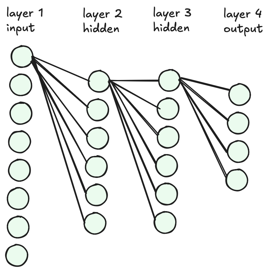
For our architecture, we’ll be using 784 input neurons (mapping directly from the 28x28 pixel grid), feeding to a first hidden layer of 128 neurons, then to a second hidden layer of 64 neurons, and finally finishing in an output layer of 10 neurons, one per digit.
There are many other network architectures we could use - and specifically for image recognition we should be using convolutions - but let’s keep it simple for our first end-to-end example.
Being a little bit more specific, we will be combining linearities and non-linearities (as an activation function) per layer. You’ll see exactly what happens in each neuron a little later.
Let’s get to some code.
Matrices
We start by defining our most important class: a matrix. You’ll often see tensors being used instead, but for this implementation we can stick with simple matrices. We keep the class itself simple, storing the data in a vector in row-major order and only having getters and setters as functions.
struct Matrix {
  int rows, cols;
  std::vector<float> data; // row major

  Matrix() : rows(0), cols(0), data(0) {}
  Matrix(int r, int c, float fill = 0.0f)
      : rows(r), cols(c), data(r * c, fill) {}

  float at(int r, int c) const { return data[r * cols + c]; } // get
  float &at(int r, int c) { return data[r * cols + c]; }      // set
};
Fun little aside: elements within a row are stored sequentially, so accessing elements in an entire row is going to have some great cache performance; accessing elements by column means constant cache misses.
We will need to define a few operations on this class. Let’s start with what we’ll need for the forward pass.
Forward pass
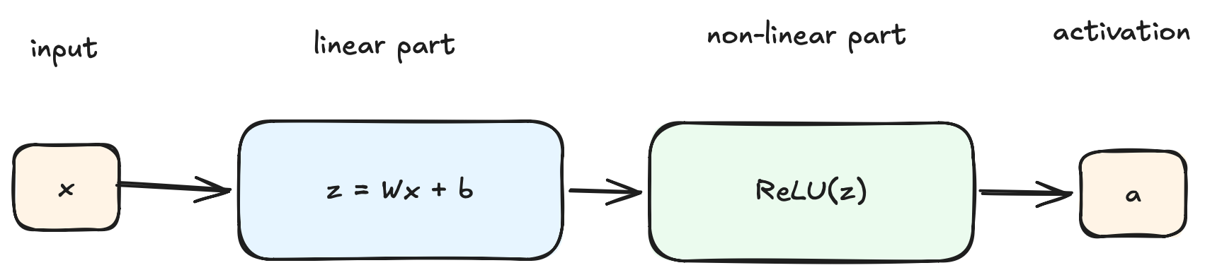
The formula for each neuron is z = Wx + b, where the weights (W) is multiplied by the input (x), with an added bias (b). This results in the pre-activation value (z): the result of linear transformation. This is then fed into an activation function / non-linear transformation - such as a ReLU operation a = ReLU(z) - in order to produce the neuron’s activation value (a).
Matrix matmul(const Matrix &A, const Matrix &B) {
  /*
  A (MxK)   B (KxN)  C (MxN)
            d e
  a b c  @  f g   =  ad+bf+ch  ae+bg+ci
            h i
  */
  Matrix C(A.rows, B.cols);

  for (int i = 0; i < A.rows; i++) {
    for (int k = 0; k < A.cols; k++) {
      float a = A.at(i, k);
      for (int j = 0; j < B.cols; j++) {
        C.at(i, j) += a * B.at(k, j);
      }
    }
  }

  return C;
}

void addBiasInPlace(Matrix &m, const Matrix &b) {
  // M: each column is one data point
  // b: 1 row only, always index at 0
  for (int c = 0; c < m.cols; c++) {
    for (int r = 0; r < m.rows; r++) {
      m.at(r, c) += b.at(0, c);
    }
  }
}

Matrix relu(const Matrix &m) {
  Matrix c(m.rows, m.cols);
  c.data = m.data; // create a copy

  for (auto &v : c.data) {
    v = std::max(0.0f, v);
  }

  return c;
}

// example for a single layer:
//   Matrix z = matmul(x, weights);
//   addBiasInPlace(z, biases);
//   Matrix a = relu(z);
This works for all but the non-linearity in the last layer. We need to turn our logits (the values of our last layer before they’re a probability) into a probability distribution so that they are all positive and sum to 1, which is where the “softmax” function comes into play. This lets us know what our model is currently predicting for a given input.
Matrix softmax(const Matrix &mIn) {
  // the stable version: subtract row max
  Matrix m(mIn.rows, mIn.cols);
  m.data = mIn.data; // create a copy

  // each row contains 1 entry
  float sum = 0.f;

  // e^i / (sum the row (e^i..N))
  for (int r = 0; r < m.rows; r++) {
    float rowMax = -999999;
    for (int c = 0; c < m.cols; c++) {
      if (m.at(r, c) > rowMax)
        rowMax = m.at(r, c);
    }

    float eSum = 0;
    for (int c = 0; c < m.cols; c++) {
      float v = m.at(r, c) - rowMax;
      float eV = std::exp(v);
      m.at(r, c) = eV;
      eSum += eV;
    }

    for (int c = 0; c < m.cols; c++) {
      m.at(r, c) /= eSum;
    }
  }

  return m;
}
That’s all we need for the forward pass. Now we should be able to have an input, pass it through various layers and get a probability at the end.
Backwards
The system wouldn’t be very interesting if all we did was a forward pass with random numbers for our weights and biases in each layer; we need to determine how we can tweak everything so that our model actually does something useful, i.e. it has to learn.
Going through the forward pass gives us a prediction. We now need a number that expresses the loss of the model (the loss function or cost function), and then we use the backwards pass to figure out how much each weight contributed to that loss in order to minimize it.
We use cross-entropy loss, which quantifies the difference between the model’s prediction probability distribution and the true labels. And seeing as we are dealing with a single-label classification model - the true class has a probability of 1, all others are 0 - the math becomes easy (this post explains it).
float crossentropySingle(std::vector<float> predictions, int indexOfCorrectClass) {
  // general cross-entropy: -sum(actual*log(predicted))
  // but we don't need it in hard labels (classification with 0/1)
  // because the 0 terms cancel out
  return -std::log(predictions[indexOfCorrectClass]);
}

float crossentropy(const Matrix &m, const std::vector<int> &indicesOfActual) {
  // indicesOfActual: array of the class (2,1,3,0,...)
  // average loss over all the batches in M (each row is 1 sample)
  float loss = 0.f;
  for (int r = 0; r < m.rows; r++) {
    float pOfCorrectClass = m.at(r, indicesOfActual[r]);
    loss += std::log(pOfCorrectClass + 1e-9f);
  }
  return -loss / (float)m.rows;
}
Now we have the loss, but we also need to understand how this fits in with training the network.
Every part that participated in the forward pass - the weights, biases, logits - needs to compute a gradient that tells us how much it contributed to the final error. This is where the chain rule comes into the picture: the output of forward pass is just a long chain of composed functions - matmul for weights, add biases, apply activation func - and we decompose the gradient calculation step by step, multiplying by the local derivative as we “unwind” all of the operations.
This mechanism is backpropagation, where the key insight is that each layer only needs to know about how its own output affects the loss. That gradient is computed from the gradient it receives from the layer above, multiplied by its own local derivative, and the multiplication chain carries this signal throughout the network.
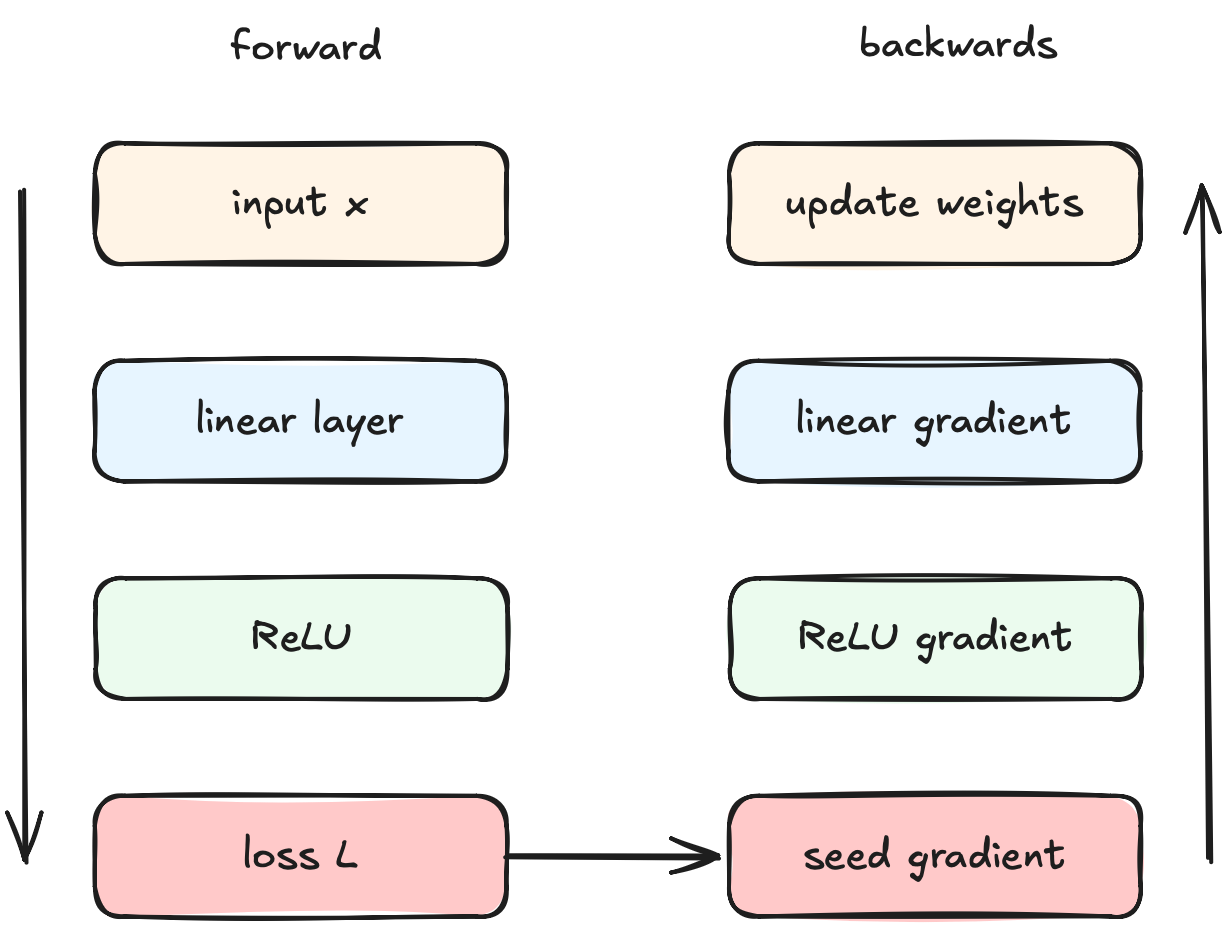
Each of the gradient components can be calculated as follows:
| Seed gradient / the starting loss | this is 1 (∂L/∂L). Cross-entropy + softmax combine to simplify it to p - y (predicted probability minus true label). |
| ReLU | either 1 or 0. If z > 0 during the forward pass, the gradient passes through unchanged. If z ≤ 0 the gradient is zero’d, as the neuron contributed nothing. |
| Weights | ∂L/∂W = δ · xᵀ - incoming signal times the input. |
| Biases | ∂L/∂b = δ - incoming signal directly. |
| Neuron activations | ∂L/∂x = Wᵀ · δ - our starting point for the next layer. |
Key: weights (W), biases (b), incoming gradient (δ), loss (L), logit (z)
Once we have calculated all the gradients, we update the weights by applying the gradients in the following manner:
W ← W − lr · ∂L/∂W- our learning rate (lr) makes us take a small step in the direction that reduces the loss. Note: If we’re smart we adjust this rate to speed up the learning, but that’s a separate topic on optimizers.
All of this requires a few more helpers in terms of code.
Matrix transpose(const Matrix &A) {
  Matrix B(A.cols, A.rows);
  for (int rA = 0; rA < A.rows; rA++) {
    for (int cA = 0; cA < A.cols; cA++) {
      B.at(cA, rA) = A.at(rA, cA);
    }
  }
  return B;
}

void axpy(float v, const Matrix &A, Matrix &B) {
  // B += v * A for applying our gradients
  for (int i = 0; i < B.data.size(); i++)
    B.data[i] += v * A.data[i];
}

void scaleInPlace(Matrix &m, float s) {
  // we need this when processing multiple batches
  // we do not want the loss to compound
  for (auto &v : m.data)
    v *= s;
}

Matrix colsum(const Matrix &m) {
  // m is (batch, # classes), b had (# classes,)
  // b is broadcast to every example in forwards,
  // backwards means sum all the gradients
  Matrix o(1, m.cols, 0.0f);
  for (int r = 0; r < m.rows; r++) {
    for (int c = 0; c < m.cols; c++) {
      o.at(0, c) += m.at(r, c);
    }
  }
  return o;
}

Matrix elemmul(const Matrix &a, const Matrix &b) {
  Matrix c(a.rows, a.cols);
  for (int i = 0; i < a.data.size(); i++)
    c.data[i] = a.data[i] * b.data[i];
  return c;
}

Matrix relugrad(const Matrix &z) {
  Matrix g(z.rows, z.cols);
  g.data = z.data;

  for (auto &v : g.data)
    v = v > 0 ? 1 : 0;

  return g;
}
Loading the data
Remember the following about matrix operations: MxK @ KxN = MxN. Or in words, in order to multiply matrix A by matrix B, matrix A’s column count needs to match matrix B’s row count.
Our weights in layer 1 go from 784 to 128, meaning we have a matrix of size 784x128. Taking a single input image means we have a matrix of size 1x784, and the output of layer 1 would result in a matrix of 1x128. However, if we were to process 8 input images, we go from 8x784 → 784x128 → 8x128.
This is pretty basic linear algebra, but it’s also pretty amazing to show how your architecture is flexible to the number of input images it can process in a batch.
Knowing that, we’re going to now write some code that starts putting everything together. We’ll be doing the following:
- Load the image data and associated correct labels into a Matrix (1 row per image) and a vector (one value per correct class of the image).
- Set up a for loop that iterates over however many epochs we want. A single epoch means we process all the training data once.
- Within each epoch, we will process a batch of samples / images instead of an individual one. This helps with computation speed, getting better gradient estimates and getting better generalization (our batches are random, introducing enough randomness to help the optimizer escape local minima). Processing the entire dataset before taking a step would be classic gradient descent, processing a single image is Stochastic Gradient Descent (SGD), and mini-batch SGD is the happy middle ground which processes a few images per step.
// data (x) stored in a single matrix (one row == 1 image)
// labels (y) stored as a list of the correct digits
Matrix xTrain = ...;
std::vector<int> yTrain = ...;
Matrix xTest = ...;
std::vector<int> yTest = ...;

std::mt19937 rng(42);

int N = xTrain.rows;
int C = xTrain.cols; // 784
int epochs = 10;
int batchSize = 64;
int numBatches = std::ceil(N / (float)batchSize);

for (int epoch = 0; epoch < epochs; epoch++) {
	// shuffle list of 0-N for batches
  std::vector<int> idx(N);
  std::iota(idx.begin(), idx.end(), 0);
  std::shuffle(idx.begin(), idx.end(), rng);

  // per minibatch - forward + backwards
  for (int b = 0; b < numBatches; b++) {
    // batch size (last batch might != batchSize if it doesn't divide nicely)
    int lastIndex = b * batchSize + batchSize;
    int currentBatchSize =
        lastIndex <= N ? batchSize : batchSize - (lastIndex - N);

    // create and populate a batch (image data and labels)
    Matrix xBatch(currentBatchSize, 784);
    std::vector<int> yBatch(currentBatchSize);
    for (int i = 0; i < currentBatchSize; i++) {
      int src = idx[b * batchSize + i];

      std::copy(xTrain.data.begin() + src * 784,
                xTrain.data.begin() + (src + 1) * 784,
                xBatch.data.begin() + i * 784);

      yBatch[i] = yTrain[src];
    }

    // now we go forwards, get loss, go backwards
}
Putting it all together
We’re getting close to having everything in place. We have the matrix, helper operations, a control flow for processing batches of data; now we just need to actually have our model and implement the forward + backward passes.
For the actual neural net definition, we just need to set up the weights and biases matrices. We will also need caches for the pre-activations and the activations for the forward + backwards passes.
  // nn architecture: 784 -> 128 -> 64 -> 10
  Matrix weights1(784, 128);
  Matrix weights2(128, 64);
  Matrix weights3(64, 10);
  Matrix biases1(1, 128, 0);
  Matrix biases2(1, 64, 0);
  Matrix biases3(1, 10, 0);
  Matrix z1Cache, z2Cache, z3Cache; // pre-activations
  Matrix a1Cache, a2Cache, a3Cache; // activations

  // init our weights
  std::mt19937 rng(42);
  heInit(weights1, rng);
  heInit(weights2, rng);
  heInit(weights3, rng);
Now for the forward + backward passes, which closely follows the logic explained above in the section.
// per minibatch - forward + backwards
for (int b = 0; b < numBatches; b++) {
  // ... as above ...

  // forward
  {
    z1Cache = matmul(xBatch, weights1); addBiasInPlace(z1Cache, biases1);
    a1Cache = relu(z1Cache);

    z2Cache = matmul(a1Cache, weights2); addBiasInPlace(z2Cache, biases2);
    a2Cache = relu(z2Cache);

    z3Cache = matmul(a2Cache, weights3); addBiasInPlace(z3Cache, biases3);
    a3Cache = softmax(z3Cache);
  }

  // loss
  {
    float l = crossentropy(a3Cache, yBatch);
    epochLoss += l;
  }

  // backwards
  {
    // layer 3
    Matrix dz3 = a3Cache;
    for (int i = 0; i < currentBatchSize; i++)
      dz3.at(i, yBatch[i]) -= 1.f; // crossentropy+softmax simplification
    scaleInPlace(dz3, 1 / (float)currentBatchSize);
    Matrix dW3 = matmul(transpose(a2Cache), dz3);
    Matrix db3 = colsum(dz3);
    Matrix da2 = matmul(dz3, transpose(weights3));

    // layer 2
    Matrix dz2 = elemmul(da2, relugrad(z2Cache));
    Matrix dW2 = matmul(transpose(a1Cache), dz2);
    Matrix db2 = colsum(dz2);
    Matrix da1 = matmul(dz2, transpose(weights2));

    // layer 1
    Matrix dz1 = elemmul(da1, relugrad(z1Cache));
    Matrix dW1 = matmul(transpose(xBatch), dz1);
    Matrix db1 = colsum(dz1);

    // apply gradients
    axpy(-lr, dW3, weights3); axpy(-lr, db3, biases3);
    axpy(-lr, dW2, weights2); axpy(-lr, db2, biases2);
    axpy(-lr, dW1, weights1); axpy(-lr, db1, biases1);
  }
}
And that’s it! While some of the functions aren’t quite trivial, I find that the control flow for what happens in training to be straightforward, helping to uncover some of the magic that you feel before checking out how things work under the hood.
I will warn you: this code is slow. Painfully slow. Add a printf for the loss calculation of each batch to see that you can’t process more than a handful each second. A single epoch on my MacBook Pro (M3 Max 40 GPU) takes roughly 1 minute. So there’s lots of room for understanding why things go so much faster if you just use PyTorch out of the box, regardless of whether using the CPU, MLX or CUDA implementation.
Check out the full code here. You’ll need this for all the MNIST and data loading, and for anything else I forgot to mention in this post.
Some closing thoughts
This code only goes through the training process - I probably should have mentioned this much sooner - and we would need a few things here to move to something more reusable: serialization of the weights + biases so that you can load them after training; implementing metrics for accuracy, confusion matrix (which digits get confused with which other digits), per-class accuracy; a simple main() that just does a forward pass on a single image.
Some more quick fire points:
- Seeing those nested loops for any of the matrix computation should make everyone’s neck hairs stand up, especially when you know that cache misses are happening all over the place when accessing things by column. This is the space I find most exciting, as it’s all just a huge learning ground for low-level hardware-specific optimization.
- There are so many other types of linear transformations we could be using. Even just moving to CNNs dramatically improves the accuracy of the model. And there are so many more things to add.
- The structure of the code is pretty explicit, but there’s something beautiful about how actual ML SDKs implement this. Plus it’s not a lot of work to have a class with a
forward()andbackward()function which abstracts everything away. - Going from this to modern LLMs is quite a jump, even without talking about the crazy scale behind the training process, or the number of parameters they use. However, looking at implementing the attention mechanism with transformers in the same manner as this post is likely going to demystify the process.